

Apr 1, 2021
Building an Electron App using Vue.js

Adam Creamer
Read More

The first beta build of Scriptless Test Automation survived thirty minutes in a customer’s hands, proving that testing AI software is a very different beast. One innocuous home-screen widget blew up the flow, and every patch we shipped uncovered a fresh cliff. Test suites were green, prospects were livid, the Board was impatient, and team morale cratered. We realized we weren’t testing software; we were mapping the behavior of a living system.
AI features live in uncharted country – no binary oracles, no neat coverage metrics, just an endless frontier of “mostly-works” edge cases. We needed a compass that could tell us how much unseen risk remained and answer the only question that mattered: “How close are we to done?”
Our compass emerged from an unlikely place: statistical species-richness estimation. By treating each new failure pattern as a “species,” Chao1 gave us a statistically defensible read on when we’d exposed enough of the unknown to ship with confidence.
What follows is how we wired Chao1 into our exploratory pipeline, the signals that matter, and why any team testing AI software needs a similar barometer for moving from testing to delivery.
Traditional software behaves like a vending machine: put in an input, expect the same candy every time. That makes binary testing natural – one scenario, one verdict, green or red. AI flips that model on its head. The algorithm is learning-based, probabilistic, and often stateful. Same input, different context, slightly different output. A single pass/fail flag can’t capture that range of behaviors.
We learned that lesson the hard way while testing AI software in Scriptless Test Automation. The first beta survived half an hour before a customer’s home-screen widget hijacked the flow and exposed a bug none of our green bars anticipated. Every hot-fix we rushed out surfaced a brand-new failure pattern. Sales saw an unending whack-a-mole; Engineering saw a matrix of permutations exploding faster than we could script; the Board saw slipping dates.
Three fault lines opened:
With every new edge case, the question grew louder: How close are we to done?
The result? False confidence when the board is watching and prospects are churning. We needed a yard-stick built for uncertainty. That’s why we turned to Chao1: instead of asking “Did every test pass?” it asks “How many undiscovered failure types still lurk out there?” – a statistical compass that finally let us make sane ship decisions in an AI world.
Chao1 was born in ecology (Elizabeth Chao, 1984) to estimate hidden species in a rainforest sample. Swap “species” for “failure patterns” and you have a practical way to ask:
“How many AI software bugs are still hiding beyond our test suite?”
Key data points:
One line of math turns a messy defect list into a single, converging metric the whole team can rally behind.

Building confidence in Scriptless Test Automation meant running it against the unknown every single day – then turning that chaos into data we could reason about. The loop we settled on is captured in Diagram 1, but the spirit matters more than the boxes and arrows: expose the engine to fresh terrain, watch where it stumbles, and convert each stumble into a signal.
We started by pulling one app at random from a pool that grew to more than a hundred titles across finance, retail, social, gaming, and a few wonderfully odd utilities. Randomization wasn’t a gimmick; it inoculated us against unconscious cherry-picking. If the algorithm was going to fail, we wanted to see it on the apps our customers might test tomorrow, not the tidy demos we’d rehearsed in the lab.
A tester spent on average 4 hours wandering the new app with human curiosity: change orientation, trigger push notifications, swipe through onboarding, add a widget, flip dark mode, kill and relaunch. Every action was captured in Kobiton’s Session Explorer and converted to a Test Case using Kobiton’s Mobile Test Management – click elements, element hierarchy, screenshots. Those trails of breadcrumbs became raw material for the next step.
With a single click, we turned the exploratory session into an automated replay: Scriptless Test Automation examined the recorded steps, inferred each selector, and attempted to replicate the flow on the same device. The beauty – and the terror – of this mechanic is that the AI makes decisions in real time. If the UI shifts even a hair, the model has to choose a new element. That’s where the interesting failures hide.
When a run went off the rails, the tester captured the artifacts – screenshots, logs, selector fields – and asked one question: Have we seen this exact failure pattern before? If they were Elizabeth Chao back in the 1980s, they would have been asking, have I seen this species of plant before?
Those counts flowed straight into a living Google Sheet. Two columns mattered most: Uniques (bugs seen only once) and Duplicates (bugs seen exactly twice). Plug those into the simple Chao1 formula and you get a lower-bound estimate of how many distinct failure types still lurk undiscovered.
Then we looped back to Step 1 with the next random app. One tester could complete one to two full cycles in a day; a small squad kept the engine humming five days a week for six straight months.

The time-series chart in the post became our morning stand-up ritual. A quick decoding:
Early on, the red band looked like a seismograph – swinging wildly as each new species moved the goalposts. But around week three a pattern emerged: blue and green kept climbing, light-green rose more slowly, and the purple line began to flatten. Most importantly, the red band narrowed from ±40% to under ±10%. That convergence did two things:
The Chao1 dashboard did more than plot curves – it put a finish line in sight. Each morning the team watched the high and low ends of the 99% confidence band inch toward one another, and morale flipped from “Will this ever end?” to “We’re closing the gap.” One engineer nailed the vibe: “It feels like we’re mining Bitcoin, but for bugs.” Every new species we uncovered pushed the estimate down and the certainty up.
Two weeks in, the convergence became unmistakable. That’s when our product manager asked the question every team secretly fears: “So…when do we stop?”
In traditional releases, the answer is binary: no open SEV-1 or SEV-2 defects, green light. But when you’re testing AI software, the world is probabilistic. We weren’t chasing absolute correctness; we were chasing a tolerable likelihood that customers wouldn’t unearth surprises we hadn’t already catalogued.
After a short but animated Zoom debate, we set a rule:
Ship when the cumulative bugs discovered equals the Chao1 point estimate and the 99 % confidence interval has effectively collapsed (high ≈ low).
In plain English: once the model predicted no more undiscovered species – and the math said the margin of error was negligible – we were done. No more whack-a-mole, just diminishing returns.
On September 10, 2024, the Android‐native line crossed that threshold. The chart looked beautiful: purple estimate flat, red and green confidence lines hugging it, light-green “Found” count touching the plateau. The team rang a virtual gong in Slack and queued the celebratory gifs.
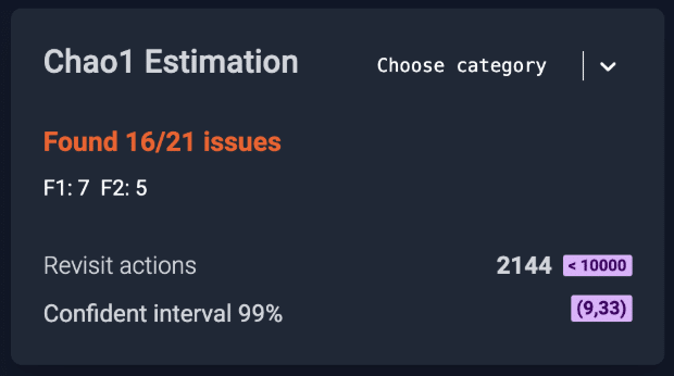
Found: shows that at this point we had unearthed 16 of the Chao1 predicted 21 bugs.
F1: 7 and F2: 5 lists the uniques (bugs seen once) and duplicates (bugs seen exactly twice) that power the Chao1 formula.
Revisit actions: Indicates that at this point we had processed 2,144 test steps in our Scriptless Test Automation.
Confidence band: Confident interval 99% of (9, 33) means the model expects the true total number of defect species to fall between 9 and 33 with 99-percent certainty.
Celebrations are fun; regressions in production, less so. I asked the crew to run ten additional random apps before we cut the build. Think of it as a statistical audit: could we add fresh evidence without moving the estimate? App #7 (the Enlighten app) broke the streak – one new species slipped through. That single data point nudged the Chao1 curve just enough to matter.
So we tightened the stop-rule:
It added three extra days and about 6,000 additional test steps, but the second run held firm. Zero new bugs, confidence interval unchanged, estimate steady. This time the gong felt earned.
Statistical stop-rules won’t give you perfection when testing AI software, but they will give you a defensible moment to move from exploration to delivery. In the messy, probabilistic world of AI features, that’s as close to certainty as product teams are likely to get – and sometimes, that’s exactly what you need to ship with confidence.
The six-month run left us with a feature users love and a repeatable playbook for anyone testing AI software. Here’s what we’d keep – and what we’d tweak – if we started tomorrow.
| Insight | Why It Matters | How To Apply |
| Visible progress fuels teams. | A shrinking confidence band gave every engineer an immediate sense of momentum. One dev compared it to “mining Bitcoin, but for bugs.” | Publish the Chao1 dashboard where everyone can see it. Let the numbers drive the stand-up, not the other way around. |
| Freeze the code until exit criteria are met. | Shipping hot-fixes mid-study skews the species counts and invalidates the estimate. | Hold all fixes behind a feature branch; merge only after you’ve cleared the stop-rule. |
| Define “bug” once–then live by it. | Inconsistent triage creates phantom species and inflates the estimate. | Draft a one-page guideline that spells out what is and isn’t a new failure pattern. Revisit only if the team hits an edge case you truly missed. |
| Beware the “Success” monoculture. | If 95% of events resolve to a single “Success” species (think a pine-tree forest), Chao1’s value drops. | Use Chao1 when failure types are sparse but meaningful. If your success rate hovers near perfection, switch to a severity-weighted metric. |
| Choose the right estimator. | Chao1 is a non-parametric richness model (Elizabeth Chao, 1984). It’s great for sparse, skewed data, but not the only game in town. | Alternatives worth exploring: Chao2 (incidence-based), ACE (Abundance-based Coverage Estimator), Jackknife 1/2, and Good-Turing. Pick the model that best fits your sample style and data distribution. |
| Create diversity in the input. | Broader input variety surfaces failure patterns your core-domain tests miss, giving Chao1 a truer read on hidden risk. | Blend daily random-app sampling with a curated set of domain-critical scenarios and track each stream in its own Chao1 panel. |
Statistical stop-rules won’t promise perfection, but they will give your team an unambiguous, data-driven moment to ship. In a world where AI behavior shifts under our feet, that kind of clarity is hard currency – worth more than Bitcoin, if you ask the team that mined those bugs. And, if you want to read more about AI in Software Testing, check out our AI in Software Testing: A Comprehensive Guide.
This snippet drops straight into any Node or browser-based tooling pipeline. Feed it a list of species (each with a name and occurrence count) and a desired confidence level; it returns Chao1’s point estimate plus upper- and lower-bounds, F1/F2 counts, and the raw species-observed metric. Because it relies only on the lightweight jstat library for z-scores, you can invoke it in a Jest test, a build-time script, or even a CI/CD step that fails the pipeline when the upper-bound exceeds your release threshold. Copy, paste, npm i jstat, and you’re in business.
import * as jst from 'jstat'

let jstat: any = jst

export interface Specie {
  specieName: string
  occurrences: number
}

export interface Chao1Data {
  species: Specie[]
  confident: number
}

export interface Chao1Result {
  Sobs: number
  chao1Number: number
  lowerBound: number
  upperBound: number
  confidentInterval: number
  F1: number
  F2: number
}

export function calculateChao1(data: Chao1Data): Chao1Result {
  const { species, confident } = data;

  const Sobs = species.length;

  const F1 = species.filter(d => d.occurrences === 1).length;
  const F2 = species.filter(d => d.occurrences === 2).length;

  let S_chao1: number;
  if (F2 === 0) {
    S_chao1 = Sobs + (F1 * (F1 - 1)) / (2 * (F2 + 1));
  } else {
    S_chao1 = Sobs + (F1 * F1) / (2 * F2);
  }

  let variance: number;
  if (F2 === 0) {
    variance = Math.pow((F1 * (F1 - 1)) / (2 * (F2 + 1)), 2);
  } else {
    variance = (F1 * (F1 - 1)) / (2 * (F2 + 1)) + Math.pow(F1, 2) * Math.pow(F1 - 1, 2) / (4 * Math.pow(F2, 2));
  }

  const standardError = Math.sqrt(variance);

  const zScore = jstat.normal.inv(1 - (1 - confident) / 2, 0, 1);

  const ciLower = S_chao1 - zScore * standardError;
  const ciUpper = S_chao1 + zScore * standardError;

  return {
    Sobs,
    chao1Number: S_chao1,
    lowerBound: ciLower,
    upperBound: ciUpper,
    confidentInterval: confident,
    F1: F1,
    F2: F2
  };
}

export function calculateMothur(data: Chao1Data): Chao1Result {
  const { species, confident } = data;
  const Sobs = species.length;
  const F1 = species.filter(d => d.occurrences === 1).length;
  const F2 = species.filter(d => d.occurrences === 2).length;

  let varChao1 = (F1 * (F1 - 1)) / (2 * (F2 + 1));
  if (F1 > 0 && F2 > 0) {
    varChao1 = (F1 * (F1 - 1)) / (2 * (F2 + 1)) +
      Math.pow(F1, 2) * Math.pow(2 * F1 - 1, 2) / (4 * Math.pow(F2 + 1, 2)) +
      Math.pow(F1, 4) * F2 * (F1 - 1) / (4 * Math.pow(F2 + 1, 3));
  } else if (F1 > 0 && F2 === 0) {
    varChao1 = (F1 * (F1 - 1)) / 2 +
      Math.pow(F1, 2) * Math.pow(2 * F1 - 1, 2) / 4 -
      Math.pow(F1, 4) / (4 * varChao1);
  } else if (F1 === 0 && F2 >= 0) {
    varChao1 = Sobs * Math.exp(-Sobs / Sobs) * (1 - Math.exp(-Sobs / Sobs));
  }

  const z = 1 + confident;
  const lowerBound = varChao1 + (F1 * (F1 - 1)) / (2 * (F2 + 1)) * Math.exp(-z * Math.sqrt(Math.log(1 + varChao1 / Math.pow(varChao1 - Sobs, 2))));
  const upperBound = varChao1 + (F1 * (F1 - 1)) / (2 * (F2 + 1)) * Math.exp(z * Math.sqrt(Math.log(1 + varChao1 / Math.pow(varChao1 - Sobs, 2))));

  return {
    Sobs,
    chao1Number: varChao1,
    confidentInterval: confident,
    lowerBound,
    upperBound,
    F1,
    F2
  };
}
Google Sheets macro
If your team lives in spreadsheets, the Apps Script macro brings Chao1 to them with zero engineering lift. Select a range containing your species IDs (one per row), call
=chao1WithCI(A2:A200, 0.99) in a cell, and Sheets returns both the estimate and the 99% confidence interval. Because everything stays inside Google Workspace, PMs and execs can tweak data, see numbers update instantly, and even chart the trend without leaving the sheet, perfect for lightweight experiments or teams without TypeScript in their stack.
function chao1WithCI(range, confidenceLevel) {
  // Get the values from the range
  const values = range.flat();

  // Count the frequency of each value
  const freqMap = {};
  values.forEach(value => {
    if (value in freqMap) {
      freqMap[value]++;
    } else {
      freqMap[value] = 1;
    }
  });

  // Calculate f1 and f2
  let f1 = 0;
  let f2 = 0;
  let observedSpecies = 0;

  for (let key in freqMap) {
    if (freqMap[key] === 1) {
      f1++;
    } else if (freqMap[key] === 2) {
      f2++;
    }
    observedSpecies++;
  }

  // Calculate Chao1
  let chao1;
  if (f2 === 0) {
    chao1 = observedSpecies + (f1 * (f1 - 1)) / 2;
  } else {
    chao1 = observedSpecies + (f1 ** 2) / (2 * f2);
  }

  // Calculate the variance for the confidence interval
  let variance;
  if (f2 === 0) {
    variance = 0;  // Cannot compute variance properly without f2
  } else {
    variance = f2 * ((f1/f2)**4 + (f1/f2)**3 + (f1/f2)**2) / 4;
  }

  // Calculate the z-score for the given confidence level
  const z = Math.abs(NormalDistInv((1 + confidenceLevel) / 2));

  // Calculate the confidence interval
  const ciLower = chao1 - z * Math.sqrt(variance);
  const ciUpper = chao1 + z * Math.sqrt(variance);

  return Chao1: ${chao1}, ${Math.round(confidenceLevel * 100)}% Confidence Interval: (${ciLower}, ${ciUpper});
}

// Function to calculate the inverse of the normal distribution
function NormalDistInv(p) {
  if (p < 0.5) {
    return -RationalApproximation( Math.sqrt(-2.0 * Math.log(p)) );
  } else {
    return RationalApproximation( Math.sqrt(-2.0 * Math.log(1.0 - p)) );
  }
}

function RationalApproximation(t) {
  const c0 = 2.515517;
  const c1 = 0.802853;
  const c2 = 0.010328;
  const d1 = 1.432788;
  const d2 = 0.189269;
  const d3 = 0.001308;
  return t - ((c2 * t + c1) * t + c0) / (((d3 * t + d2) * t + d1) * t + 1.0);
}

